Price elasticity of demand can be measured by three methods. They are:
- Total Expenditure or Outlay Method:
In this method, the total expenditure on the quantity of a commodity demanded is used to find out whether the total expenditure has increased or decreased or constant, consequent on the changes in its price. In the first case, consequent on the fall in price from Rs.6 to Rs.5 and then to Rs.4, the quantities demanded have increased to 1500 and 2000 respectively. Due to the fall in price, the total outlay has gone up. So, when the total outlay increases due to a fall in price the demand is elastic. In the second case, total outlay remains constant irrespective of changes in prices and hence the demand is of unit elasticity. In the third case, total outlay decreases with the fall in price. So, it has an inelastic demand. In the figure, the AB portion of the total expenditure curve slopes downward showing, as the price falls, the total expenditure is increasing and vice versa. So, the demand at this price range is elastic and Ep is greater than 1. Over the price range from OP2 to OP3 the total expenditure curve shows that as the price falls, the expenditure decreases and as the price increases from OP3 to OP2, the total expenditure increases showing that the demand is inelastic and Ep is smaller than one. In the price range P1 to P2, the total expenditure does not change. Hence, the elasticity is unity and Ep = 1.
Price (in Rs / Kg) Quantity Demanded (in Quintals) Total Expenditure or Outlay in Purchasing that Quantity (Rs) Elasticity
- 6.00 1000 6000 Elastic Demand Ep >1
5.00 1500 7500
4.00 2000 8000
- 6.00 1000 6000 Unit Elasticity Ep = 1
5.00 1200 6000
4.00 1500 6000
III 6.00 1000 6000 Inalastic Demand Ep < 1
5.00 1100 5500
4.00 1300 5200
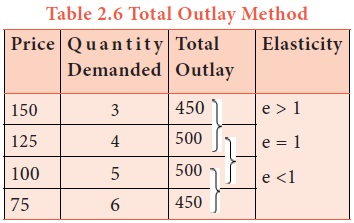
Fig: Elasticity of Demand-Total Outlay or Expenditure Method
- Measuring Elasticity at a Point:
When the price falls from OP0 to OP1, the quantity demanded increases from OQ0 to OQ1. Using the formula, elasticity of demand is given by:
Ep = (Proportionate change in quantity demanded) / (Proportionate change in price) Fig: Equation of point elasticity

Fig: Elasticity of Demand: Point Method
In the figure a, the triangle K0RK1 is similar to triangle K0Q0T and, therefore,
Canceling Q0 K0 on both sides, we get Ep = Q0 T /O Q0. The assumption is that a very small change in price and quantities has been considered and so, points K0 and K1 on tT lie very close so as to almost coincide. If this be the assumption, then Q0 K0 should coincide with Q1 K1 and in right-angled triangle tOT, the relation Q0T / OQ0 can be expressed as TK0 / K0t. Since TK0 is the lower sector of the demand curve at this point and K0t is its upper sector, we can say that in a demand curve at any point,
Elasticity = (Lower sector) / (Upper Sector) That is, Elasticity at point K0 = K0T / K0t
At point K, in Figure b, the lower and upper sectors are equal and hence, at K, the demand is unitary elastic. And point below K, say L, will show inelastic demand and any point above K, say M will show elastic demand. At the point where the demand curve touches the X-axis, the value of Ep = 0 (perfectly inelastic), and at the point where the demand curve touches the Y-axis the value of Ep is ∝ (infinite) (perfectly elastic).
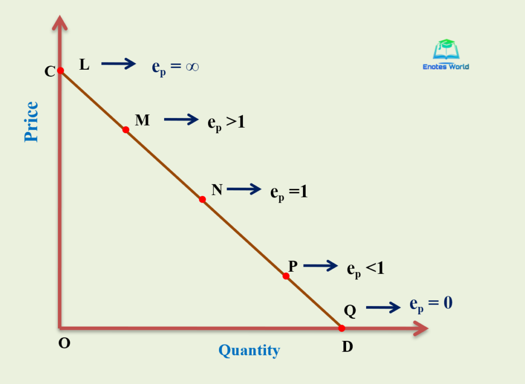
Fig b: Price Elasticity of Demand: Point Method
- Arc Method:
The Point Method of Elasticity of demand studied above refers to the condition where the price changes and in quantities demanded are very small so that we can find out the elasticity at a point. Since the changes are very little, we take the original price and quantity as the basis of measurement. Suppose, the change in price and quantity is very large, neither the initial nor final price and quantities can be taken.
Price (Rs/Kg) Quantity Demanded (Kgs/Day)
30 200
20 400
Ep = (200/200) X (30/10) = 3 Instead, suppose we take final price and quantity demanded, then the elasticity is EP = (200/400) X (20/10) =1.
Now, there is a wide difference in elasticities, if we take initial or final prices. Hence, arc elasticity of demand is used to solve this problem. For this, the average of both initial and final prices and quantities are used.
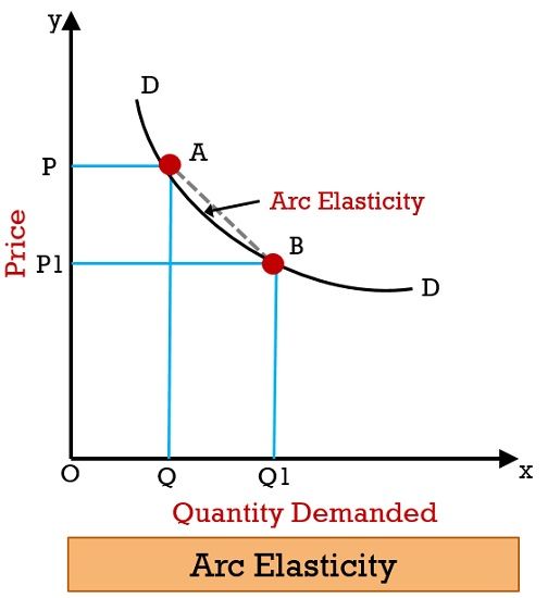
Fig: Elasticity of Demand-Arc Method